kirra-docs
Time Window Dialog
The Time Window dialog is Kirra’s timing-and-vibration analysis surface. It groups seven tabs over a shared blast-pattern scope so you can move between event histograms, frequency content, waveform synthesis, and detune actions without losing the selection you’re analysing.
The dialog is opened from the Analyse toolbar (the Time Window, FFT, Spectrum, Seed, Forward Array, Detune and Constrain button — see Analyse Toolbar).
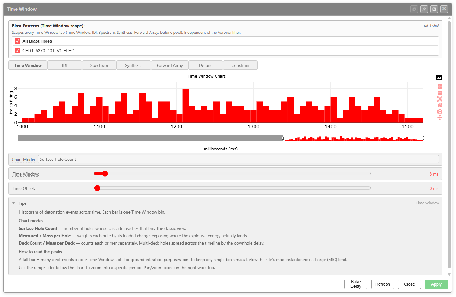 The Time Window tab — histogram of detonation events with chart-mode selector, Time Window slider, Time Offset slider, and the in-app Tips panel.
Shared layout
Every tab shares the same wrapper:
| Region | Purpose |
|---|---|
| Title bar | Always reads Time Window. Dock, pin, minimise, and close controls on the right |
| Blast Patterns (Time Window scope) | Per-entity checkboxes — picks which blast patterns feed every tab in the dialog. The header notes Scopes every Time Window tab (Time Window, IDI, Spectrum, Synthesis, Forward Array, Detune pool). Independent of the Voronoi filter. |
| Tabs | Time Window, IDI, Spectrum, Synthesis, Forward Array, Detune, Constrain |
| Tab body | Chart + tab-specific controls |
| Tips panel | Collapsible help text written into the app, specific to the active tab |
| Footer buttons | Bake Delay, Refresh, Close, Apply (the Apply button is renamed Apply Detune on the Detune tab) |
The scope panel is independent of the Voronoi monitor filter — what you tick here is what every chart in the dialog operates on.
Time Window tab
Histogram of detonation events across time. Each bar is one Time Window bin.
Controls
| Control | Purpose |
|---|---|
| Chart Mode | Choose how each event is weighted: Surface Hole Count, Measured / Mass per Hole, or Deck Count / Mass per Deck |
| Time Window slider | Bin width in milliseconds. Default shown above is 8 ms |
| Time Offset slider | Shifts the bins along the time axis. Default 0 ms |
| Rangeslider under the chart | Zoom into a specific period; pan/zoom icons on the right work too |
Chart modes (verbatim from the in-app Tips)
- Surface Hole Count — number of holes whose cascade reaches that bin. The classic view.
- Measured / Mass per Hole — weights each hole by its loaded charge, exposing where the explosive energy actually lands.
- Deck Count / Mass per Deck — counts each primer separately. Multi-deck holes spread across the timeline by the downhole delay.
How to read the peaks
A tall bar = many deck events in one Time Window slot. For ground-vibration purposes, aim to keep any single bin’s mass below the site’s max-instantaneous-charge (MIC) limit.
IDI tab (Inter-Detonation Interval)
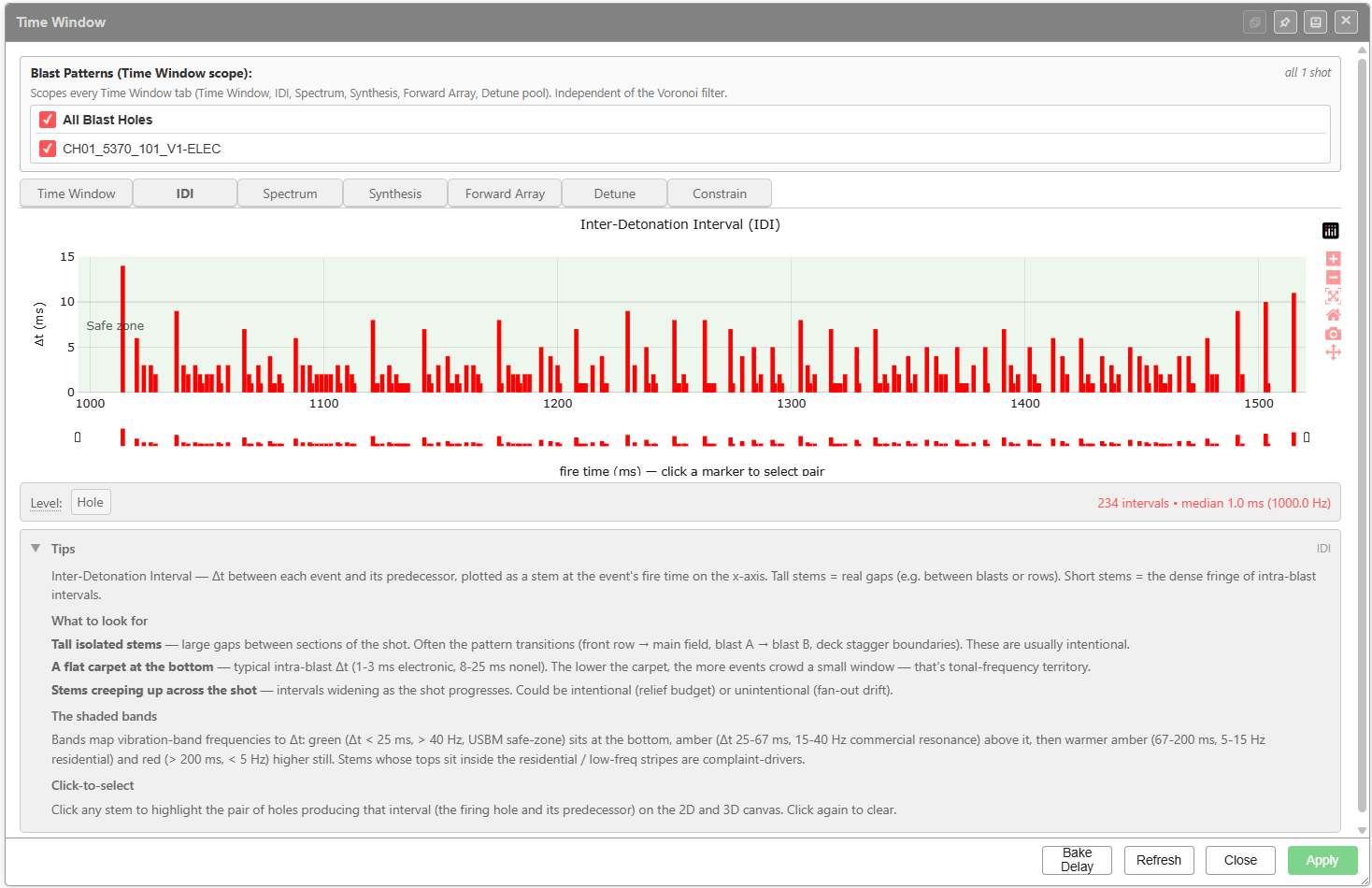
Δt between each event and its predecessor, plotted as a stem at the event’s fire time on the x-axis. Tall stems = real gaps (e.g. between blasts or rows). Short stems = the dense fringe of intra-blast intervals.
Controls
| Control | Purpose |
|---|---|
| Level | Granularity of the interval calculation. The screenshot shows Hole |
What to look for (verbatim from the in-app Tips)
- Tall isolated stems — large gaps between sections of the shot. Often the pattern transitions (front row → main field, blast A → blast B, deck stagger boundaries). These are usually intentional.
- A flat carpet at the bottom — typical intra-blast Δt (1-3 ms electronic, 8-25 ms nonel). The lower the carpet, the more events crowd a small window — that’s tonal-frequency territory.
- Stems creeping up across the shot — intervals widening as the shot progresses. Could be intentional (relief budget) or unintentional (fan-out drift).
The shaded bands
Bands map vibration-band frequencies to Δt: green (Δt < 25 ms, > 40 Hz, USBM safe-zone) sits at the bottom; amber (Δt 25-67 ms, 15-40 Hz commercial resonance) above it; then warmer amber (67-200 ms, 5-15 Hz residential); and red (> 200 ms, < 5 Hz) higher still. Stems whose tops sit inside the residential / low-freq stripes are complaint-drivers.
Click-to-select
Click any stem to highlight the pair of holes producing that interval (the firing hole and its predecessor) on the 2D and 3D canvas. Click again to clear.
Spectrum tab (FFT of Impulse Train)
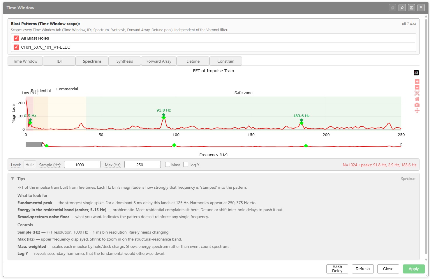
FFT of the impulse train built from fire times. Each Hz bin’s magnitude is how strongly that frequency is “stamped” into the pattern.
Controls
| Control | Purpose |
|---|---|
| Level | Source granularity — Hole in the screenshot |
| Sample (Hz) | FFT resolution. 1000 Hz = 1 ms bin resolution. Rarely needs changing |
| Max (Hz) | Upper frequency displayed. Shrink to zoom in on the structural-resonance band |
| Mass (checkbox) | Mass-weighted. Scales each impulse by hole/deck charge — shows energy spectrum rather than event-count spectrum |
| Log Y (checkbox) | Log Y axis — reveals secondary harmonics the fundamental would otherwise dwarf |
Reading the chart (verbatim from the in-app Tips)
- Fundamental peak — the strongest single spike. For a dominant 8 ms delay this lands at 125 Hz. Harmonics appear at 250, 375 Hz etc.
- Energy in the residential band (amber, 5-15 Hz) — problematic. Most residential complaints sit here. Detune or shift inter-hole delays to push it out.
- Broad-spectrum noise floor — what you want. Indicates the pattern doesn’t reinforce any single frequency.
Frequency-band colouring
| Band | Label | Typical concern |
|---|---|---|
| Pink/red | Low freq | Below structural resonance — building sway |
| Amber | Residential | 5-15 Hz residential building resonance |
| Light amber | Commercial | Commercial structures, 15-40 Hz |
| Green | Safe zone | Above structural resonance |
The peak readout at the bottom (e.g. peaks: 91.8 Hz, 2.9 Hz, 183.6 Hz) lists the strongest peaks across the displayed range.
Synthesis tab
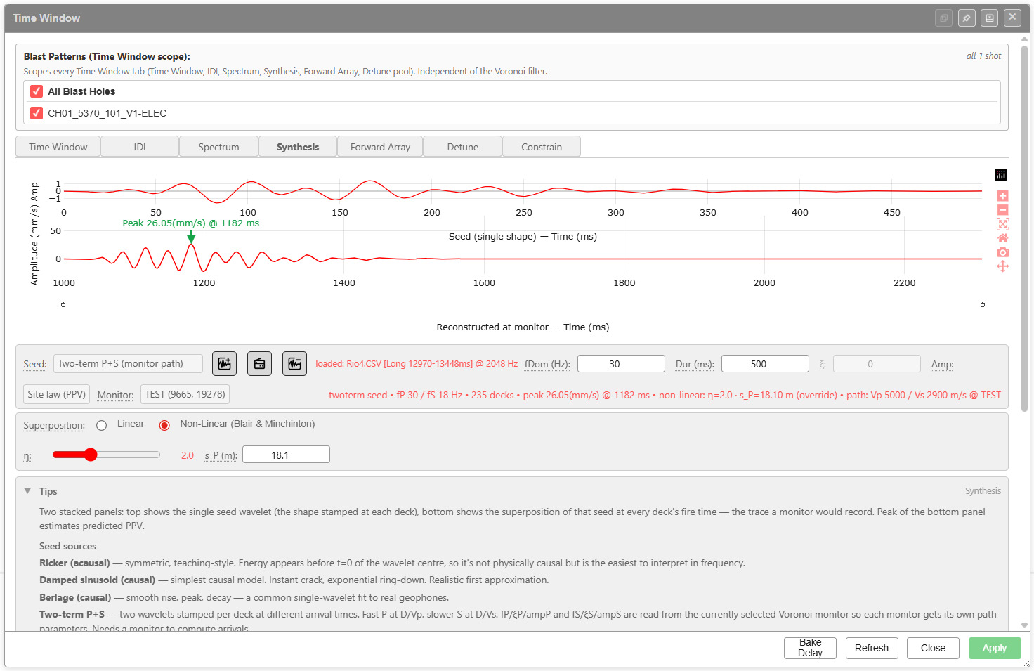
Two stacked panels: top shows the single seed wavelet (the shape stamped at each deck); bottom shows the superposition of that seed at every deck’s fire time — the trace a monitor would record. Peak of the bottom panel estimates predicted PPV.
Controls
| Control | Purpose |
|---|---|
| Seed | Source wavelet shape. Options include Two-term P+S (monitor path), Ricker (acausal), Damped sinusoid (causal), Berlage (causal), plus loaded seed files. The three buttons next to the dropdown are seed-library actions [VERIFY: button labels for the three icons next to the Seed dropdown] |
| fDom (Hz) | Dominant frequency of the seed |
| Dur (ms) | Duration of the seed window |
| ξ | Damping parameter (active for damped seeds) |
| Amp | Amplitude scale |
| Site law (PPV) | Site-law profile used for amplitude scaling |
| Monitor | The Voronoi monitor that defines the receptor position and site-law constants |
| Superposition | Linear or Non-Linear (Blair & Minchinton) |
| η (non-linear only) | Non-linearity exponent. Range slider with numeric readout |
| s_P (m) (non-linear only) | P-wave saturation distance override |
Seed sources (verbatim from the in-app Tips)
- Ricker (acausal) — symmetric, teaching-style. Energy appears before t=0 of the wavelet centre, so it’s not physically causal but is the easiest to interpret in frequency.
- Damped sinusoid (causal) — simplest causal model. Instant crack, exponential ring-down. Realistic first approximation.
- Berlage (causal) — smooth rise, peak, decay. A common single-wavelet fit to real geophones.
- Two-term P+S — two wavelets stamped per deck at different arrival times. Fast P at D/Vp, slower S at D/Vs. fP / ξP / ampP and fS / ξS / ampS are read from the currently selected Voronoi monitor so each monitor gets its own path parameters. Needs a monitor to compute arrivals.
Status readout
The red line under the seed selector reports the current physics, e.g. twoterm seed • fP 30 / fS 18 Hz • 235 decks • peak 26.05(mm/s) @ 1182 ms • non-linear: η=2.0 · s_P=18.10 m (override) • path: Vp 5000 / Vs 2900 m/s @ TEST.
Forward Array tab
Three-component (L / T / V) wave synthesis at a monitor with optional Love-wave packet in the T component. The chart stacks L (longitudinal / radial), T (transverse), and V (vertical) with the peak of each labelled.
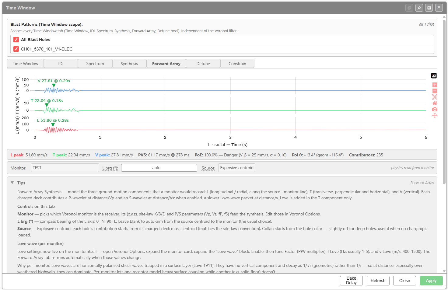
Controls (verbatim from the in-app Tips)
- Monitor — picks which Voronoi monitor is the receiver. Its (x,y,z), site-law K/B/E, and P/S parameters (Vp, Vs, fP, fS) feed the synthesis. Edit those in Voronoi Options.
- L brg (°) — compass bearing of the L axis: 0=N, 90=E. Leave blank to auto-aim from the source centroid to the monitor (the usual choice).
- Source — Explosive centroid: each hole’s contribution starts from its charged-deck mass centroid (matches the site-law convention). Collar: starts from the hole collar — slightly off for deep holes, useful when no charging is loaded.
Love wave (per monitor)
Love settings now live on the monitor itself — open Voronoi Options, expand the monitor card, expand the Love wave block. Enable, then tune Factor (PPV multiplier), f Love (Hz, usually 1-5), and v Love (m/s, 400-1500). The Forward Array tab re-runs automatically when those values change.
Status readout
Bottom band reports peaks and risk metrics in this order:
L peak • T peak • V peak • PVS (peak vector sum @ time) • PoE (probability of exceedance with V_β / σ) • Pol θ (geometric polarisation angle) • Contributors (number of decks summed)
The polarisation Pol θ is reported as geom (signed) — for example Pol θ: -13.4° (geom -116.4°).
Why per-monitor Love settings
Love waves are horizontally polarised shear waves trapped in a surface layer (Love 1911). They have no vertical component and decay as 1/√r (geometric) rather than 1/r — so at distance, especially over weathered highwalls, they can dominate. Per-monitor lets one receptor model heavy surface coupling while another (e.g. solid floor) doesn’t.
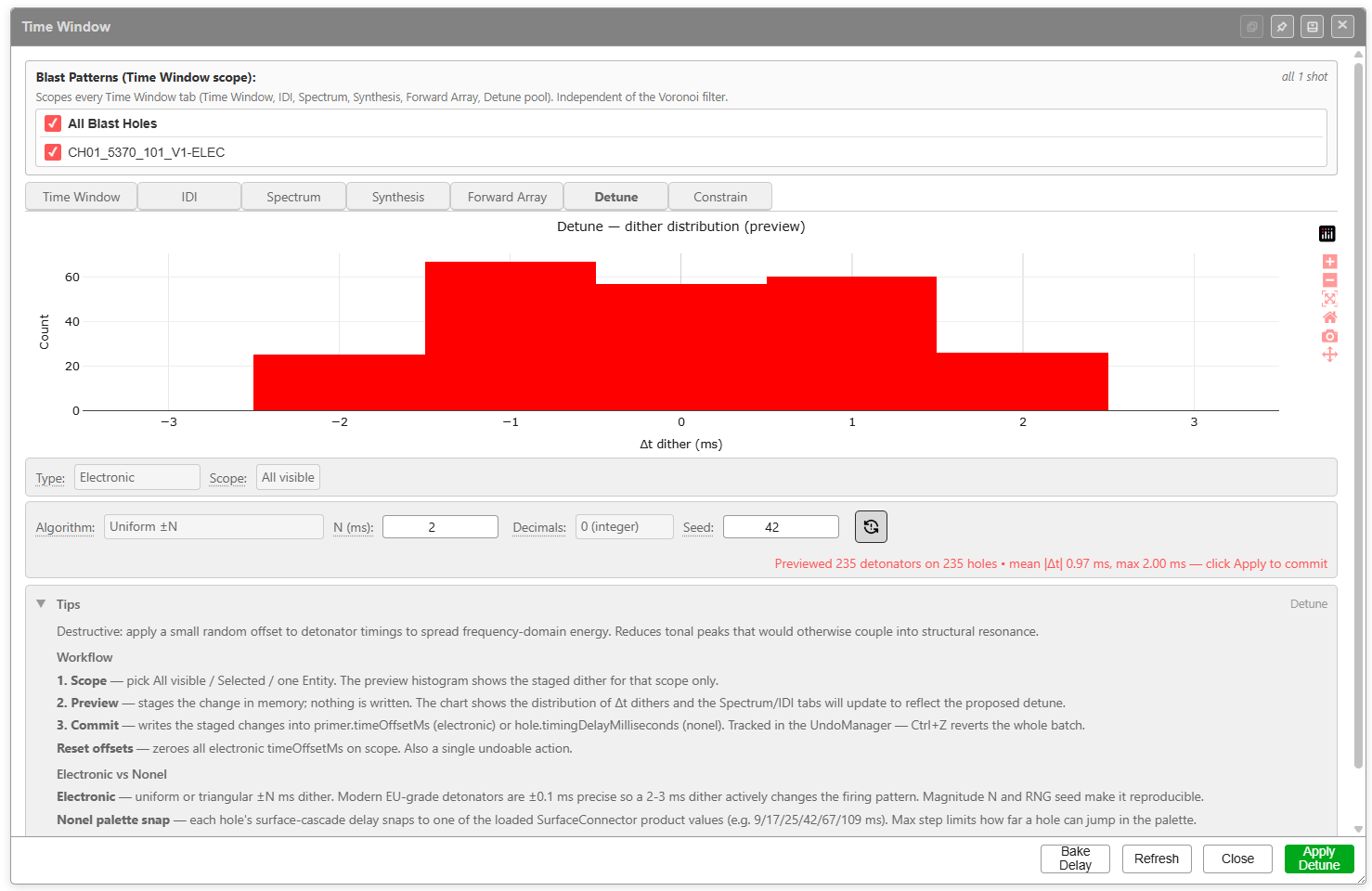
Detune tab
Apply a small random offset to detonator timings to spread frequency-domain energy. Reduces tonal peaks that would otherwise couple into structural resonance.
Controls
| Control | Purpose |
|---|---|
| Type | Electronic or Nonel — chooses which timing field the dither writes to |
| Scope | All visible, Selected, or one Entity — limits which holes are affected |
| Algorithm | Uniform ±N or other distribution. The chart previews the staged Δt distribution |
| N (ms) | Magnitude of the dither |
| Decimals | Rounding (the screenshot shows 0 (integer)) |
| Seed | RNG seed for reproducibility (default 42) |
| Refresh icon next to Seed | Re-rolls the seed and re-previews |
| Apply Detune | Commits the staged dither (the right-hand footer button changes from Apply to Apply Detune on this tab) |
Workflow (verbatim from the in-app Tips)
- Scope — pick All visible / Selected / one Entity. The preview histogram shows the staged dither for that scope only.
- Preview — stages the change in memory; nothing is written. The chart shows the distribution of Δt dithers and the Spectrum/IDI tabs will update to reflect the proposed detune.
- Commit — writes the staged changes into
primer.timeOffsetMs(electronic) orhole.timingDelayMilliseconds(nonel). Tracked in the UndoManager —Ctrl+Zreverts the whole batch.
Reset offsets — zeroes all electronic timeOffsetMs on scope. Also a single undoable action.
Electronic vs Nonel
- Electronic — uniform or triangular ±N ms dither. Modern EU-grade detonators are ±0.1 ms precise so a 2-3 ms dither actively changes the firing pattern. Magnitude N and RNG seed make it reproducible.
- Nonel palette snap — each hole’s surface-cascade delay snaps to one of the loaded SurfaceConnector product values (e.g. 9 / 17 / 25 / 42 / 67 / 109 ms). Max step limits how far a hole can jump in the palette.
Status readout
| After preview the dialog reports *Previewed N detonators on M holes • mean | Δt | X ms, max Y ms — click Apply to commit*. |
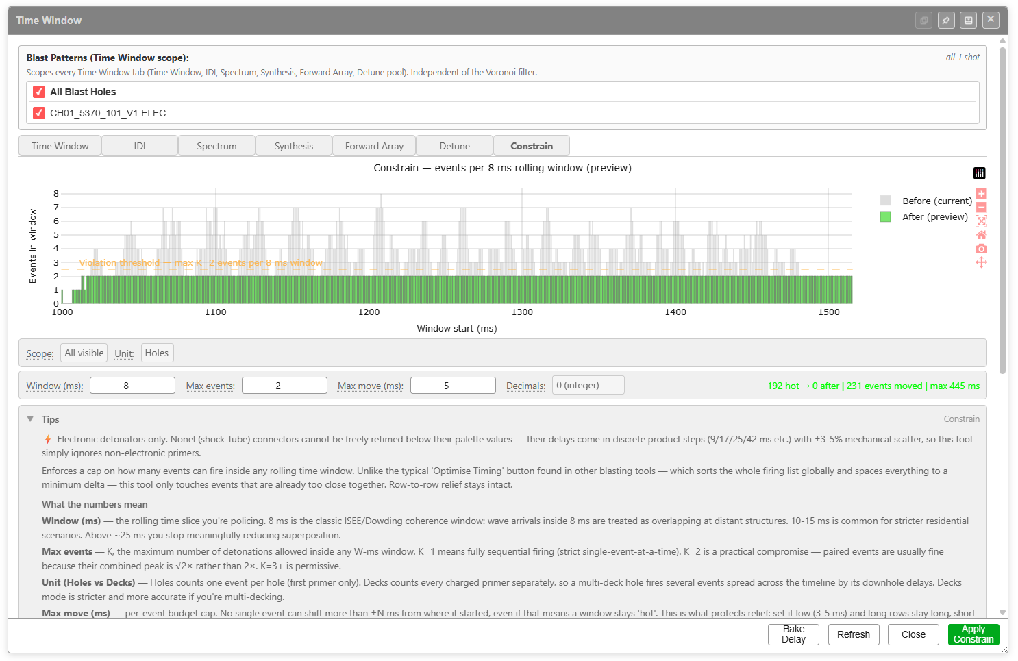
Constrain tab
Event-rate enforcement — flag events that fall inside a rolling window (preview, with Before and After counts in the legend). The current screenshot is small; the controls visible are Scope, Level, Window (ms), Max events, and Max move (ms).
[SCREENSHOT NEEDED: high-resolution Constrain tab so each control and its tooltip are legible]
What this tab does [VERIFY: full Constrain workflow and what “constrain” writes]
From the in-app Tips visible in the screenshot:
Electronic detonators only. Nonel (shock-tube) connectors cannot be freely detuned below their palette values — their delays come in discrete product steps (9/17/25/42/etc) so a >50 ms mechanical solder, so the tool simply ignores non-electronic primers.
The constrain operation appears to detect and reduce window violations by rescheduling electronic detonators within an allowable jitter (Max move (ms)) so that no rolling-window slot exceeds Max events. The chart shows the rolling-window event count before and after, and tall green stems are violations.
Suggested workflow [VERIFY: against current build]
- Set Scope and Level (Hole / Deck)
- Set the Window (ms) — the rolling time window inside which events are counted
- Set Max events — the cap per window
- Set Max move (ms) — the maximum jitter the constrainer is allowed to introduce
- Preview reports N violations and visualised before/after
- Click Apply to commit (the change is written into electronic
timeOffsetMsand is undoable as one batch)
Bake Delay
The Bake Delay button at the bottom of the dialog folds any active electronic offsets (timeOffsetMs) and detune/constrain results into the underlying timing field so the staged values become the new baseline.
This is the same Bake-onto-Electronic action used in the Connect Toolbar.
[VERIFY: exact behaviour of Bake Delay button when triggered from the Time Window dialog footer vs the Connect toolbar]
Related topics
- Analyse Toolbar — opens this dialog
- Analytics Overview — GPU shader models and Voronoi PPV
- PPV & Vibration Models — the underlying site law and waveform models
- PPV Voronoi Modes — per-cell receptor-aware PPV
- Electronic Timing Constructs — where
timeOffsetMsis written - Connect Toolbar — Bake onto Electronic Detonators